Why is FAT Slow on SD Card?

This article discusses the performance limitations of the FAT file system with a focus on SD Card. After a brief refresher on FAT fundamentals, we show how FAT predictably achieves high access performances in the absence of fragmentation, but how fragmentation can build up until performances suddenly collapse. We conclude with a few important recommendations.

FAT Fundamentals

In FAT file systems, files are divided in equally sized blocks called clusters which are allocated as files grow. Contiguous clusters (in file order) need not be contiguously stored on disk. Instead, the logical file order is separately maintained in a dedicated on-disk table called the file allocation table (FAT). The \(k^{th}\) entry of the file allocation table contains the next (in file order) physical cluster number (effectively, its address on disk) after cluster number \(k\). This effectively creates a linked list of clusters referred to as a cluster chain.

From an algorithmic performance standpoint, the cluster chain comes with linear time complexity. This is neither good or bad in and of itself, although it does become a problem when it compounds with an unfortunate consequence of the FAT allocation scheme: fragmentation.

The Best Case Scenario

First consider an ideal scenario: a file is created in an otherwise empty file system and appended with new data until it reaches some target size. In that case, the resulting cluster layout would resemble that of Figure 1, where logically contiguous clusters (in file order) end up contiguous on disk as well. In theory, some implementation could produce something radically different, but it would make little sense to deviate substantially from the natural allocation order assumed here.

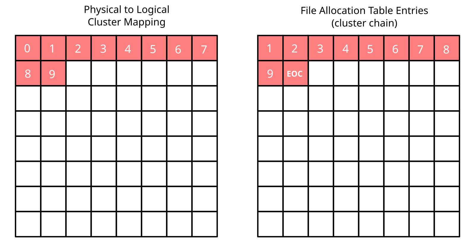
Example diagram representation of a File Allocation Table (FAT) with a single unfragmented cluster chain.

The allocation scenario depicted in Figure 1 is ideal in terms of access performance. Contiguous clusters allow for large sequential accesses, which are always faster than small scattered accesses on SD card. Most importantly, the cluster chain is stored in a very compact manner, FAT entries occupying the lowest possible number of sectors.

With a typical 4KiB sector containing 4096 / 4 = 1024 FAT entries (assuming FAT32), sequential accesses to a non-fragmented file will produce a negligible one FAT sector read per 1024 clusters of accessed data overhead. This is assuming minimal caching, that is, a single read buffer.

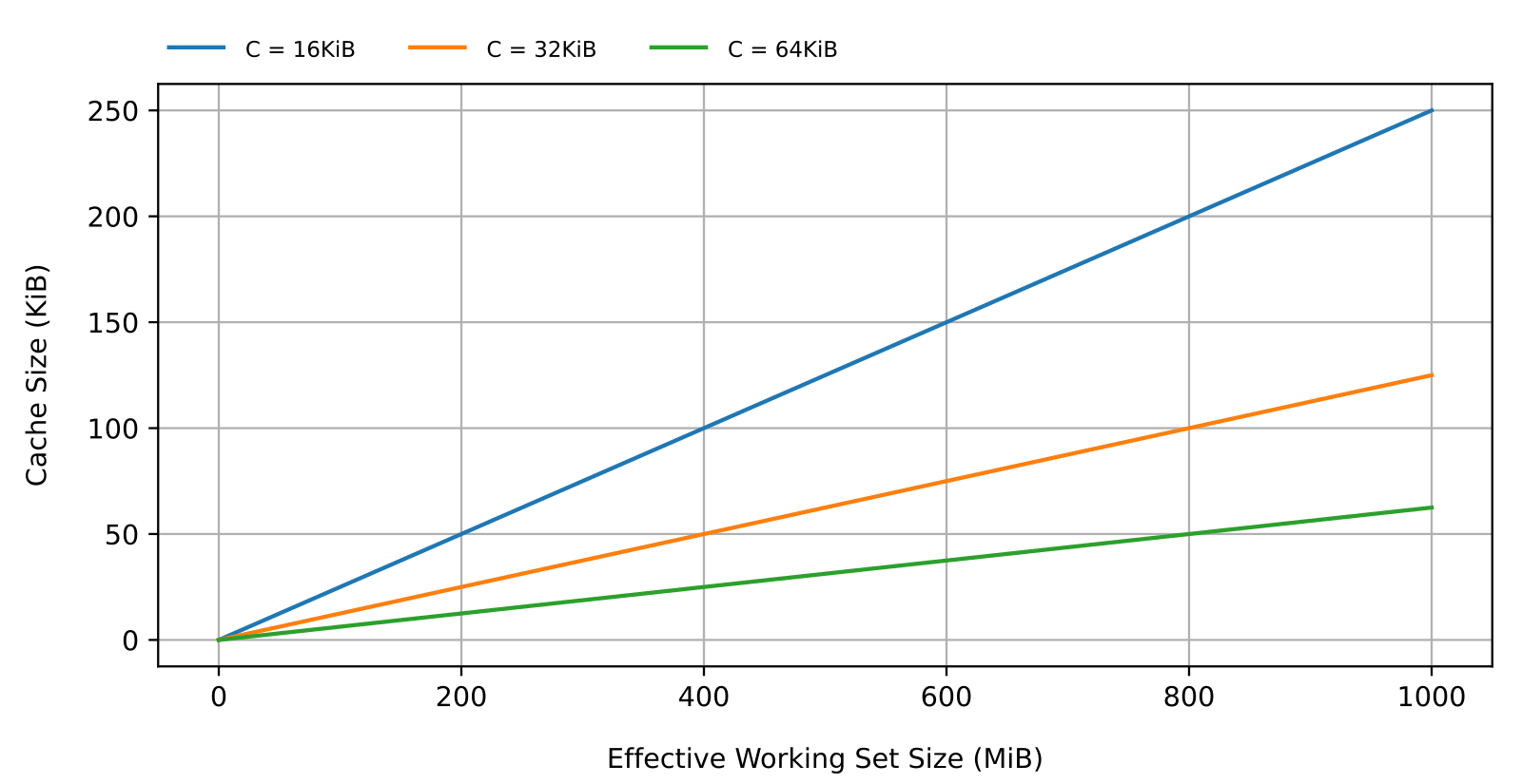
The absence of fragmentation is also beneficial to random access performances as it makes for efficient caching (greater spatial locality). As the working set increases, caching needs to grow at the same rate to maintain the highest access throughput, which may or may not become a problem depending on the size of the working set and the amount of RAM available (and the anticipated level of fragmentation as we will see shortly). Assuming FAT32, the cache size \(H\) needed to maximize throughput (100% cache hits) with a working set size \(W\) and a cluster size \(C\) is

\(H = \frac{4W}{C} \quad . \tag {1}\)

Figure 2 shows how cache requirements increase as working sets get larger. Notice the variety of RAM requirements. Notice also the impact of the cluster size. Larger clusters come with lower RAM usage at the potential cost of less efficient disk usage. This can be a problem for applications dealing with a large number of small files.

Line graph of the effective working set in MiB that can fit in cache for three different cluster size. — **Figure 2 –** Cache size needed to maintain maximum performances based on the size of the working set.

Performances with Fragmentation

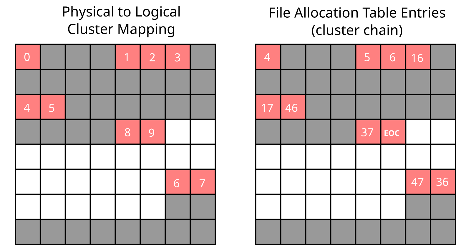
Now consider a different scenario where, instead of appending data to a single file, multiple files are written at arbitrary positions, extended, truncated and occasionally deleted or created. In that more complex scenario, the resulting file layout could resemble that of Figure 3, where clusters from a same file are spread across the whole disk. This is an example of fragmentation. With fragmentation, caching gets statistically less efficient, the absolute worst case being that a chain with \(N\) clusters resides in \(N\) different FAT sectors.

Example diagram of a File Allocation Table (FAT) with a fragmented cluster chain. — **Figure 3 –** Sequential file allocation in a half-full file system. The focus is on one file (shown in red). Clusters belonging to other files are shown in gray.

In the case of sequential accesses, there is really no reasons for performances to be dramatically affected by fragmentation. In the worst case (with a cluster chain spread over \(N\) sectors), only one extra FAT sector read per cluster is needed, which is not too bad.

For random-like accesses, we start with equation 2 and introduce fragmentation in the form of a fragmentation factor \(F\). \(F\) is the ratio between the number of FAT sectors needed for storing a cluster chain, and the minimum number of FAT sectors that would be needed in the absence of fragmentation. The cache requirement then becomes

\(H = \frac{4WF}{C} \quad . \tag {2}\)

The level of fragmentation and the size of the working set can be the lumped into a single metric \(L = WF\), which can be interpreted as the effective size of the working set given the presence of fragmentation. Using this model, more fragmentation or more data has the same effect on performance so, from now on, when we refer to the size of the working set, we always refer to the effective size unless specified otherwise.

Fragmentation can dramatically and unpredictably increase over time. When the level of fragmentation exceeds a certain threshold the cache becomes too small for the (effective) working set, and gets continuously trashed through successive travels along the cluster chain. This essentially neutralize the cache, leading to a sudden collapse in access throughput.

Without cache, we assume that each arbitrary access requires half of the cluster chain to be browsed on average. This is somewhat of a pessimistic assumption given that a lookup should not start back from the first cluster when an access is performed farther down the chain (relative to the previous access). We nonetheless accept the assumption for the sake of simplicity and because it is largely irrelevant to our conclusions. The throughput \(\omega\) is given by

\(\omega = \frac{A}{T_L + T_A} \tag {3}\)

where \(A\) is the access size, \(T_L\) is the lookup time and \(T_A\) the access time. Without cache, the half-chain travel time is

\(T_L = \frac{2 L T_R}{CS} \tag {4}\)

where \(L\) is the effective size of the working set, \(T_R\) the sector read time, \(C\) the cluster size, and \(S\) the sector size. Combining equation 3 and 4, we get

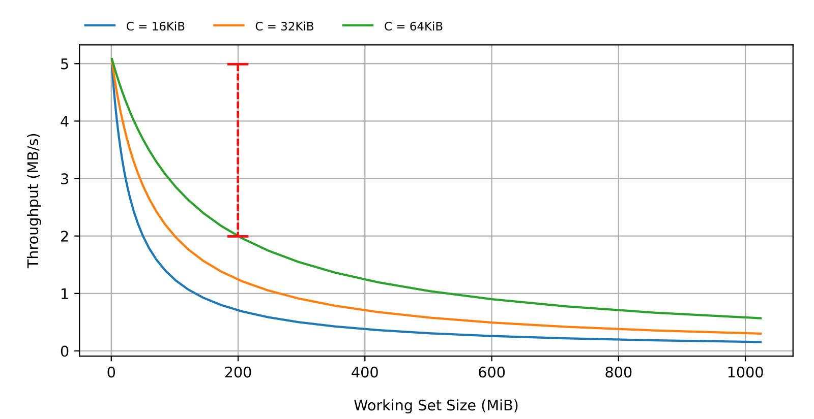
\(\omega = \frac{ACS}{2LT_R + T_ACS} \tag {5}\)

which is shown in Figure 4 as a function of \(L\), for different cluster sizes, and with \(S=A=4096\) bytes and \(T_R=T_A=1\) millisecond. Looking at Figure 4 we can determine the amount of performance degradation to expect, when the size of the working set exceeds the capacity of the cache to absorb the lookup overhead. For instance, given a 200MiB working set, the average throughput would fall from 5MB/s to 2MB/s with 16KiB clusters (shown in red).

Read performance in MB/s versus the working set size without caching for three different cluster size. — **Figure 4 –** Read performances as a function of the effective working set size without cache.

Takeaways

For a mostly sequential workload, fragmentation is not much of a problem. Even if the file allocation is complex enough that it does create fragmentation, further accesses should only be marginally affected.
Whenever possible, use fallocate to pre-allocate entire files and avoid file deletion and truncation.
For more complex and unpredictable workloads, make sure to carefully balance performance, RAM, access pattern and data size, keeping in mind that fragmentation can slowly appear with time, increasing the effective size of the working set, and possibly neutralizing the effect of the cache.

One final word of caution

FAT uses in-place updates for both user data and internal metadata. It is partly why FAT access performances are at their best (including for random-like accesses) on non-fragmented files. The flip side of in-place updates, though, is that they are hard to reconcile with raw flash, on one hand, and fail-safe operation, on the other hand.

For raw flash compatibility, FAT needs an extra flash translation layer (FTL) to bridge the gap between the block device interface expected by FAT and the more complex reality of raw flash devices (see What is a Flash File System). To provide fail-safety, a journal, or some other retrofitted fail-safe mechanism, must be added. In both cases, performances and resource requirements can be heavily impacted and additional performance implications can only be dealt with on an individual implementation basis.

This is where a more modern transactional flash file system like TSFS makes things much easier. TSFS supports all flash devices, including SD card, eMMC, raw NOR and raw NAND devices. It is inherently fail-safe and is insensitive to fragmentation, providing the highest possible level of performance regardless of the access workload.

If you want to learn more about TSFS, please head on to the TSFS product page. In the meantime, thank you for reading. If you have any questions regarding embedded file systems or any other embedded-related topic, please feel free to reach out to us.